Orr Sommerfeld pseudospectra

Let’s use the classic Orr-Sommerfeld problem to explore pseudospectra with Dedalus.

The Orr-Sommerfeld problem explores the stability of flow down a rectangular channel driven by a pressure gradient. The equilibrium solution is known analytically as plane Poiseuille flow, and is given by

\[U(z) = 1 - z^2.\]

This shear flow becomes unstable despite having no inflection point in the flow. This is in contradiction to Rayleigh’s inflection point theorem, which states that a necessary condition (for a sufficient condition, see Balmforth and Morrison (1998)). for a shear flow in an inviscid fluid to become unstable, it must have a point \(z_i\) with

\[\frac{d^2 U}{dz^2}(z_i) = 0.\]

This means that for plane Poiseuille flow, the viscosity itself is the source of the instability.

If we write the problem in canonical Dedalus form

\[\mathcal{M}\frac{\partial \mathbf{X}}{\partial t} + \mathcal{L} \mathbf{X} = N(\mathbf{X}),\]

linearize about \(U(z)\) such that \(N(\mathbf{X}) = 0\), and take the time dependence of \(\mathbf{X} \propto e^{-ict}\), we have a generalized eigenvalue problem.

This is a very interesting problem because the linear operator for the Orr-Sommerfeld problem \(\mathcal{L}_{OS}\) is non-normal, that is \(\mathcal{L}_{OS}^\dagger \mathcal{L}_{OS} \neq \mathcal{L}_{OS}\mathcal{L}_{OS}^\dagger\). Non-normal operators can drive transient growth: even systems in which all eigenmodes are linearly stable and will decay to zero, arbitrary initial conditions can be amplified by large factors.

Here, we assume perturbations take the form \(u(x,z,t) = \hat{u} e^{i\alpha (x - ct)}\), where \(c = \omega/\alpha\) is the wave speed. One must take care to note that \(c = c_r + i c_i\). If a perturbation has \(c_i > 0\), it will linearly grow. This occurs at a Reynolds number \(\mathrm{Re} \simeq 5772\), a result you can also find using CriticalFinder (it’s actually a test problem for eigentools).

However, as we will see below, even at \(\mathrm{Re} = 10000\), the growth rate is tiny: \(c_i \approx 3.7\times10^{-3}\)! Yet at those Reynolds numbers, channel flow is clearly unstable. How can this be?

The answer is that the spectrum of the Orr-Sommerfeld operator is quite misleading. Because \(\mathcal{L}_{OS}\) is non-normal, its eigenfuntions are not orthogonal. As they decay at different rates, the total amplitude of some arbitrary initial condition can increase!

This observation was first noted in the pioneering paper by Reddy, Schmid, and Henningson (1993). For a detailed discussion of the Orr-Sommerfeld problem including a thorough discussion of transient growth, see Schmid and Henningson (2001).

import matplotlib.pyplot as plt
from mpi4py import MPI
from eigentools import Eigenproblem, CriticalFinder
import dedalus.public as de
import numpy as np
import time

Orr-Sommerfeld problem

First, we’ll define the Orr-Sommerfeld equation in the usual way (following Orszag 1971), in which the Navier-Stokes equations are reduced to a single fourth-order differential equation for the wall-normal velocity \(w\). Because of the first order form of dedalus, this becomes four first order equations.

Then we create an Eigenproblem object.

z = de.Chebyshev('z', 128)
d = de.Domain([z],comm=MPI.COMM_SELF)

alpha = 1.
Re = 10000

orr_somerfeld = de.EVP(d,['w','wz','wzz','wzzz'],'c')
orr_somerfeld.parameters['alpha'] = alpha
orr_somerfeld.parameters['Re'] = Re
orr_somerfeld.substitutions['umean']= '1 - z**2'
orr_somerfeld.substitutions['umeanzz']= '-2'

orr_somerfeld.add_equation('dz(wzzz) - 2*alpha**2*wzz + alpha**4*w -1j*alpha*Re*((umean-c)*(wzz - alpha**2*w) - umeanzz*w) = 0')
orr_somerfeld.add_equation('dz(w)-wz = 0')
orr_somerfeld.add_equation('dz(wz)-wzz = 0')
orr_somerfeld.add_equation('dz(wzz)-wzzz = 0')

orr_somerfeld.add_bc('left(w) = 0')
orr_somerfeld.add_bc('right(w) = 0')
orr_somerfeld.add_bc('left(wz) = 0')
orr_somerfeld.add_bc('right(wz) = 0')

# create an Eigenproblem object
EP = Eigenproblem(orr_somerfeld)

2021-02-01 17:21:04,593 problems 0/1 INFO :: Solving EVP with homogeneity tolerance of 1.000e-10
2021-02-01 17:21:04,613 problems 0/1 INFO :: Solving EVP with homogeneity tolerance of 1.000e-10

Eigenmode rejection

Calling the solve method on the Eigenproblem object will solve the eigenvalue problem with 128 modes and then solve it again with \(3/2 \cdot 128 = 192\) modes. Using the rejection algorithm detailed in Chapter 7 of Boyd (1989), eigentools creates EP.evalues which holds only the good eigenvalues: those that are the same (to some specified tolerance) between both solves.

Of course, EP.evalues_low and EP.evalues_high store the low and high resolution eigenvalues, respectively, if you need them.

The sparse=False option tells Dedalus to use the dense eigenvalue solver, which will retrieve all the eigenmodes (as many as there are modes in the problem). Of course, about half of them will be unusably inaccurate; the rejection methods in eigentools hides those from us.

EP.solve(sparse=False)

Plotting Spectra

eigentools has the ability to make simple spectra automatically:

ax = EP.plot_spectrum()

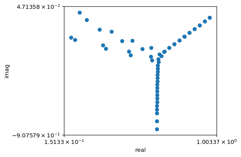
By default, this plotting tool uses double-log plotting (that is, it logs positive and negative values separately); while it is highly configurable, sometimes it’s easiest to simply make a plot manually using the real and imaginary parts of the eigenvalues themselves. Because we’re going to overplot pseudospectra later, it’s easier to use this approach here.

Below, we use standard matplotlib plotting tools to construct a simple spectrum with a horizontal line at the stability threshold.

plt.scatter(EP.evalues.real, EP.evalues.imag,color='red')
plt.axis('square')
plt.axhline(0,color='k',alpha=0.2)
plt.xlim(0,1)
plt.ylim(-1,0.1)
plt.xlabel(r"$c_r$")
plt.ylabel(r"$c_i$")

Text(0, 0.5, '$c_i$')

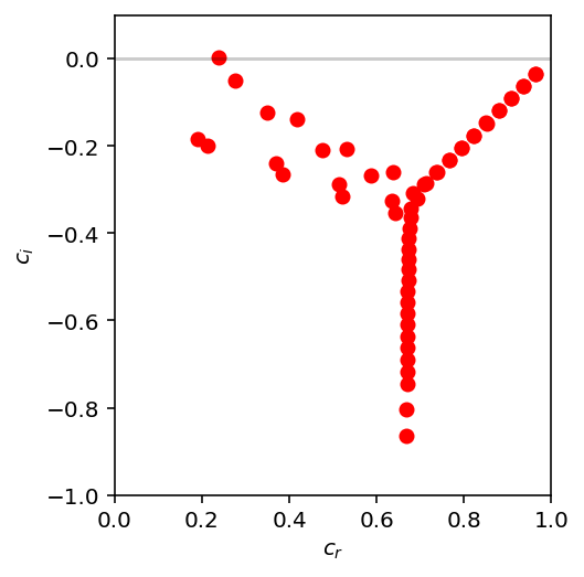
We can find the growth rate also:

print(r"fastest growth rate: max(c_i) = {:5.3e}".format(np.max(EP.evalues.imag)))

fastest growth rate: max(c_i) = 3.740e-03

Pseudospectra

The Eigenproblem object also provides a simple method to calculate pseudospectra, calc_ps(). Pseudospectra were originally defined for regular eigenvalue problems. In order to calculate pseudospectra for the differential-algebraic equation systems Dedalus typically provides, we use the algorithm developed by Embree and Keeler (2017). This uses the sparse eigenvalue solver to construct an invariant subspace to approximate a regular eigenvalue problem. Typically, it requires a rather high number of modes, \(k\). Here we set \(k = 100\). After we construct the approximate matrix, we feed it to a standard pseudospectrum routine. This requres a set of points in the complex plane at which the pseudospectrum will be computed. We do that by choosing a set of real and imaginary points, and feeding them to the EP.calc_ps() method.

k = 100

psize = 100
real_points = np.linspace(0,1, psize)
imag_points = np.linspace(-1,0.1, psize)

Choosing an inner product and norm

The concept of non-normality is inherently linked to the norm used to evaluate orthogonality. When calculating pseudospectra, one must specify the norm to be used.

eigentools allows users to pass a norm function to the pseudospectrum calculation. If you do not pass a norm, it will simply use the standard vector 2-norm in the coffiecient space. This is almost assuredly unphysical. However, it is simple to write a function to use the energy norm (or anything else).

Here, we will use the energy inner product for the Orr-Sommerfeld form of the equations,

\[<\mathbf{X}_1|\mathbf{X}_2>_E = \int_{-1}^{1} w_1^\dagger w_2 + \frac{(\partial_z w_1)^\dagger \partial_z w_2}{\alpha^2} dz,\]

with \(\mathbf{X}_{1,2}\) state vectors containing \(w\) and its first three derivatives. This inner product induces a norm \(||\mathbf{X}||_E\) that is equal to the energy of the perturbation.

The input to the functions will be Dedalus FieldSystem objects which will be populated by EP.calc_ps(). Note that the function returns the energy itself, that is it calls field['g'][0] to return the integral in grid space.

def energy_norm(X1, X2):
    u1 = X1['wz']/alpha
    w1 = X1['w']
    u2 = X2['wz']/alpha
    w2 = X2['w']

    field = (np.conj(u1)*u2 + np.conj(w1)*w2).evaluate().integrate()
    return field['g'][0]

Now we can call calc_ps with the points we defined above and energy_norm:

EP.calc_ps(k, (real_points, imag_points), inner_product=energy_norm)

This adds data attributes EP.pseudospectrum, EP.ps_real, EP.ps_imag to the EP object, storing the pseudospectrum contours, and the real and imaginary grid for conveninece.

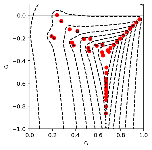
Traditionally, one plots pseudospectra as logarithmic contours over top of the spectrum. Here, the contours are from -1 to -8 from outside in. This means that a perturbation of amplitude \(\epsilon \simeq 10^{-1}\) to \(\epsilon \simeq 10^{-8}\) will cause an \(\mathcal{O}(1)\) change in the eigenvalues within that contour. Importantly, transient growth is possible within all of the contours that cross \(c_i > 0\) with amplification factors proportional to \(1/\epsilon\). Here, we can clearly see why channel flow is turbulent even when the only unstable mode has such a feeble growth rate!

plt.scatter(EP.evalues.real, EP.evalues.imag,color='red')
plt.contour(EP.ps_real,EP.ps_imag, np.log10(EP.pseudospectrum),levels=np.arange(-8,0),colors='k')
plt.axis('square')
plt.axhline(0,color='k',alpha=0.2)

plt.xlim(0,1)
plt.ylim(-1,0.1)
plt.xlabel(r"$c_r$")
plt.ylabel(r"$c_i$")

Text(0, 0.5, '$c_i$')

Primitive Form

One of the great advantages of Dedalus is that we can study problems without having to manipulate them into special forms, as in the case of the Orr-Sommerfeld operator. After all, this is nothing more than a special form of the 2-D Navier-Stokes equation linearized around \(U(z)\).

We should be able to enter the “primitive” form of the equations and get equivalent results. Here, we define a new Dedalus EVP, and then feed it to eigentools.

primitive = de.EVP(d,['u','w','uz','wz', 'p'],'c')
primitive.parameters['alpha'] = alpha
primitive.parameters['Re'] = Re

primitive.substitutions['umean'] = '1 - z**2'
primitive.substitutions['umeanz'] = '-2*z'
primitive.substitutions['dx(A)'] = '1j*alpha*A'
primitive.substitutions['dt(A)'] = '-1j*alpha*c*A'
primitive.substitutions['Lap(A,Az)'] = 'dx(dx(A)) + dz(Az)'

primitive.add_equation('dt(u) + umean*dx(u) + w*umeanz + dx(p) - Lap(u, uz)/Re = 0')
primitive.add_equation('dt(w) + umean*dx(w) + dz(p) - Lap(w, wz)/Re = 0')
primitive.add_equation('dx(u) + wz = 0')
primitive.add_equation('uz - dz(u) = 0')
primitive.add_equation('wz - dz(w) = 0')
primitive.add_bc('left(w) = 0')
primitive.add_bc('right(w) = 0')
primitive.add_bc('left(u) = 0')
primitive.add_bc('right(u) = 0')


prim_EP = Eigenproblem(primitive)

2021-02-01 17:21:40,598 problems 0/1 INFO :: Solving EVP with homogeneity tolerance of 1.000e-10
2021-02-01 17:21:40,648 problems 0/1 INFO :: Solving EVP with homogeneity tolerance of 1.000e-10

Again, we solve the dense eigenproblem just to get the full spectrum.

prim_EP.solve(sparse=False)

And we recalculate the pseudospectrum, covering the same part of the complex plane.

However, the energy norm in primitive variables is slightly different:

\[<\mathbf{X}_1|\mathbf{X}_2>_E = \int_{-1}^{1} u_1^\dagger u_2 + w_1^\dagger w_2 dz,\]

so we write another energy_norm function and then call prim_EP.calc_ps with the same arguments as before.

def energy_norm(Q1, Q2):
    u1 = Q1['u']
    w1 = Q1['w']
    u2 = Q2['u']
    w2 = Q2['w']

    field = (np.conj(u1)*u2 + np.conj(w1)*w2).evaluate().integrate()
    return field['g'][0]

prim_EP.calc_ps(k, (real_points, imag_points), inner_product=energy_norm)

Now, let’s plot both the Orr-Sommerfeld form and the primitive form.

clevels = np.arange(-8,0)
OS_CS = plt.contour(EP.ps_real,EP.ps_imag, np.log10(EP.pseudospectrum),levels=clevels,colors='blue',linestyles='solid', alpha=0.5)
P_CS = plt.contour(prim_EP.ps_real,prim_EP.ps_imag, np.log10(prim_EP.pseudospectrum),levels=clevels,colors='red',linestyles='solid', alpha=0.5)

plt.scatter(prim_EP.evalues.real, prim_EP.evalues.imag,color='red',zorder=3)
plt.scatter(EP.evalues.real, EP.evalues.imag,color='blue',marker='x',zorder=4)

lines = [OS_CS.collections[0],P_CS.collections[0]]
labels = ['O-S form', 'primitive form']

plt.axis('square')
plt.xlim(0,1)
plt.ylim(-1,0.1)
plt.axhline(0,color='k',alpha=0.2)
plt.xlabel(r"$c_r$")
plt.ylabel(r"$c_i$")
plt.legend(lines, labels)
plt.tight_layout()
plt.savefig("OS_pseudospectra.png", dpi=300)

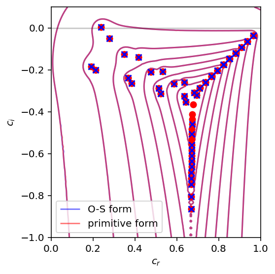
We see that the on the whole, there is very good agreement. The primitive form has more good eigenvalues (red dots with no corresponding blue crosses; none of the converse). Furthermore, the pseudospectra contours are indistinguishable except in the lower branch around \((c_r, c_i) = (0.65,-0.8)\).