Mixed Layer Instability

This notebook implements the eigenvalue problem posed in

Boccaletti, Ferrari, & Fox-Kemper, 2007: Journal of Physical Oceanography, 37, 2228-2250.

This demonstrates the use of the grow_func option to Eigenproblem to specify a custom calculation method for determining the growth rate of a given eigenvalue.

This script also gives an example of using project_mode to compute a 2D visualization of the most unstable eigenmode.

import numpy as np
import matplotlib.pylab as plt
from eigentools import Eigenproblem, CriticalFinder
import dedalus.public as de
from dedalus.extras import plot_tools

# problem parameters
kx = 0.8  # x-wavelength
ky = 0    # y-wavelength
δ = 0.1   # Prandtl ratio f/N
Ri = 2    # Richardson number
L = 1     # Characteristic length scale along front
Hy = 0.05 # Vertical scale
ΔB = 10   # Buoyancy jump at bottom of mixed layer

# discretization parameters
nz = 32
nx = 32 # only necessary for 2D visualization

# Only need the z direction to compute eigenvalues
z = de.Chebyshev('z',nz, interval=[-1,0])
d = de.Domain([z], grid_dtype=np.complex128)

evp = de.EVP(d, ['u','v','w','p','b'],'sigma')

evp.parameters['Ri'] = Ri
evp.parameters['δ'] = δ
evp.parameters['L'] = L
evp.parameters['Hy'] = Hy
evp.parameters['ΔB'] = ΔB
evp.parameters['kx'] = kx
evp.parameters['ky'] = ky
evp.substitutions['dt(A)'] = '1j*sigma*A'
evp.substitutions['dx(A)'] = '1j*kx*A'
evp.substitutions['dy(A)'] = '1j*ky*A'
evp.substitutions['U'] = 'z + L'

evp.add_equation('dt(u) + U*dx(u) + w - v + Ri*dx(p) = 0')
evp.add_equation('dt(v) + U*dx(v)     + u + Ri*dy(p) = 0')
evp.add_equation('Ri*δ**2*(dt(w) + U*dx(w)) - Ri*b  + Ri*dz(p) = 0')
evp.add_equation('dt(b) + U*dx(b) - v/Ri + w = 0')
evp.add_equation('dx(u) + dy(v) + dz(w) = 0')

evp.add_bc('right(w) = 0')
evp.add_bc('left(w + dt(p/ΔB) - Hy*v) = 0')

2021-02-01 17:21:18,102 problems 0/1 INFO :: Solving EVP with homogeneity tolerance of 1.000e-10

Specifying a definition of stability

Because the notion of stability depends on the assumed time dependence and there are several widely used conventions, eigentools allows users to define what “growth” and “frequency” mean in the context of their problem. This is done by passing grow_func and freq_func to Eigenproblem. These functions take a complex number z and return the “growth” and “frequency” corresponding to it.

In this problem the time dependence is given by

\[e^{i \sigma t},\]

so the growth rate is \(-Im(\sigma)\) and the frequency is \(Re(\sigma)\).

g_func = lambda z: -z.imag
f_func = lambda z: z.real
EP = Eigenproblem(evp, grow_func=g_func, freq_func=f_func)

2021-02-01 17:21:18,137 problems 0/1 INFO :: Solving EVP with homogeneity tolerance of 1.000e-10

The EP.growth_rate() method will provide the eigenvalue corresponding to the fastest growing mode, as defined by grow_func. Here, we use sparse=False because this is an ideal problem with many exactly zero eigenvalues, the fastest growing mode is never closest to zero. Thus, we must either provide a guess or use the dense solver.

rate, indx, freq = EP.growth_rate(parameters={'Hy':Hy, 'kx': kx}, sparse=False)
print("fastest growing mode: {} @ freq {}".format(rate, freq))

fastest growing mode: 0.19931003960491872 @ freq -0.33556838187371807

EP.growth_rate also provides indx, which is the index to the most unstable eigenmode. We can then use that to access that eigenmode for visualization.

Plotting eigenmodes

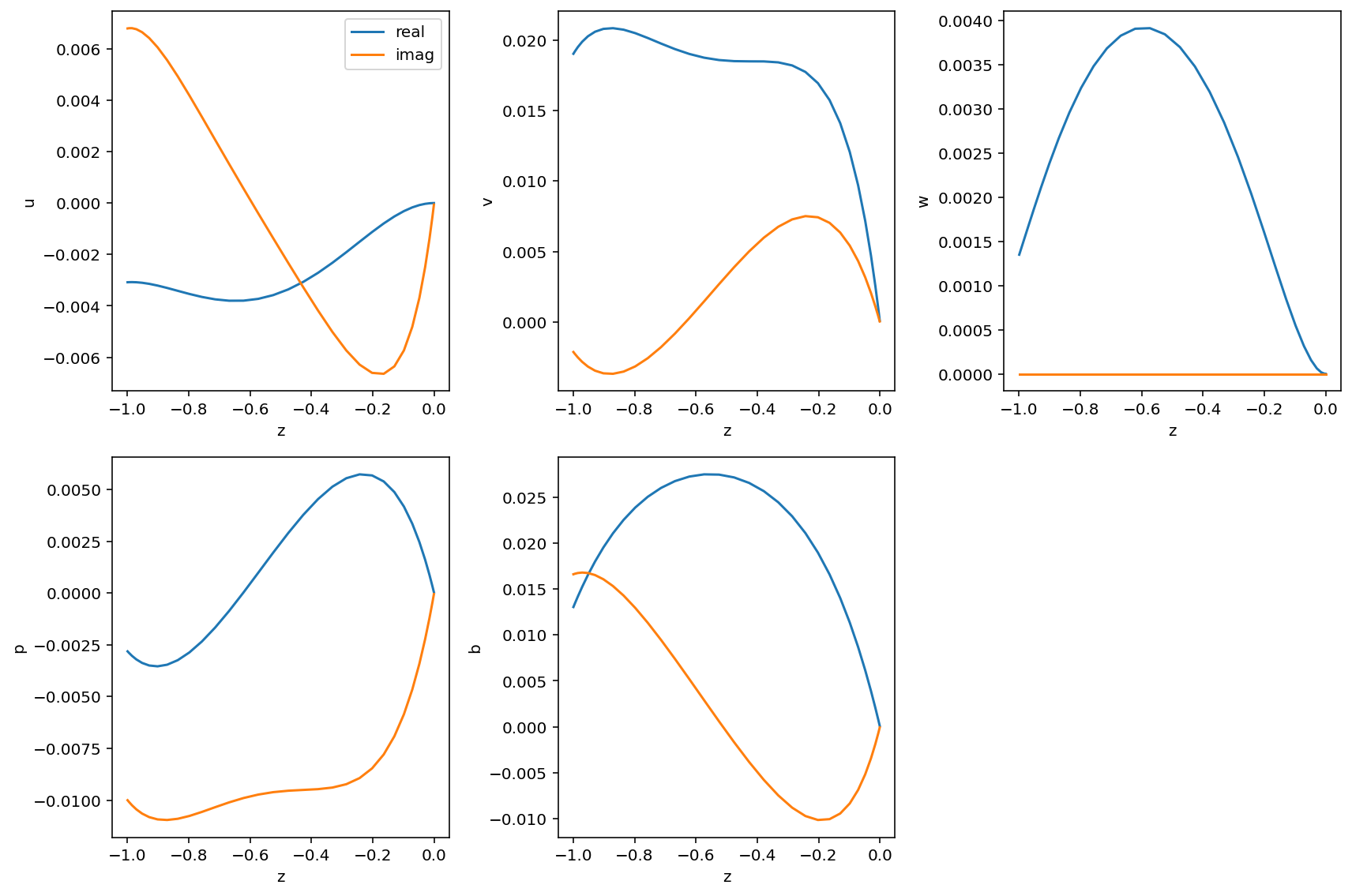
Because the eigenvalue problems solved by Dedalus are one-dimensional, eigentools provides a simple method to visualize all of the modes. In general, these solutions are complex, with the real and imaginary parts of each variable determining their phase relationships. Because eigenmodes are only defined to a relative phase, EP.plot_mode allows the user to specify a variable to normalize against. All variables are multiplied by the complex conjugate of the chosen mode. Here, we have chosen the vertical velocity w. Note that its plot shows no imaginary part.

fig = EP.plot_mode(indx, norm_var='w')
fig.savefig('mixed_layer_unstable_1D.png')

Projection onto higher dimensional domains

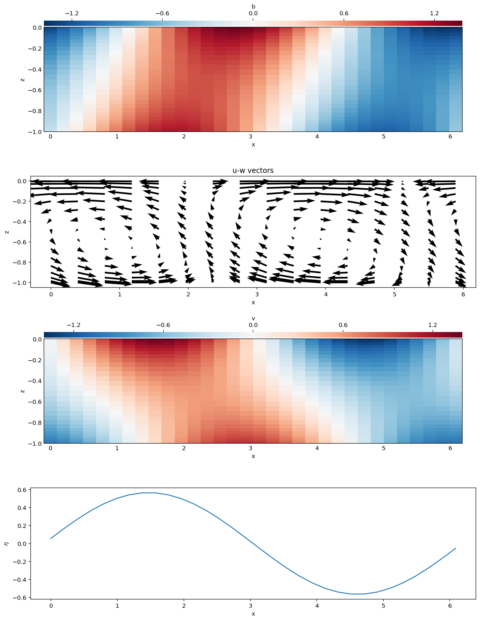
However, because this is a 2-D problem with \(e^{i k x}\) dependence in \(x\), we often want to visualize this mode in 2-D also. In order to do so, we define a 2-D domain using Dedalus with the \(x\) direction added. Note that this domain has a grid dtype of np.float64 because once we project against the complex exponential in \(x\), the various fields in the eigenmode become real variables.

# define a 2D domain to plot the eigenmode
x = de.Fourier('x',nx)
d_2d = de.Domain([x,z], grid_dtype=np.float64)

Next we will produce a 2-D plot of the most unstable eigenmode shown in figure 7 from Boccaletti, Ferrari, and Fox-Kemper (2007).

First we must project the eigenmode against the 2-D domain using EP.project_mode. Again we specify the mode index using indx and then specify the transverse mode; here we choose 1 so that we do not need to scale \(L_x\).

fs = EP.project_mode(indx, d_2d, (1,))

EP.project_mode() returns a Dedalus FieldSystem object holding all of the variables in the problem. It can then be accessed using the familiar fs['u']['g'] interface to get the grid space representation of the x-velocity \(u\).

Below, we use Dedalus’s plot_tools to help generate the plots.

scale=2.5
nrows = 4
ncols = 1
image = plot_tools.Box(4, 1)
pad = plot_tools.Frame(0.2, 0.2, 0.1, 0.1)
margin = plot_tools.Frame(0.3, 0.2, 0.1, 0.1)
mfig = plot_tools.MultiFigure(nrows, ncols, image, pad, margin, scale)
fig = mfig.figure

for var in ['b','u','v','w','p']:
    fs[var]['g']

# b
axes = mfig.add_axes(0,0, [0,0,1,1])
plot_tools.plot_bot_2d(fs['b'], axes=axes)

# u,w
axes = mfig.add_axes(1,0, [0,0,1,1])
data_slices = (slice(None), slice(None))
xx,zz = d_2d.grids()
xx,zz = np.meshgrid(xx,zz)
axes.quiver(xx[::2,::2],zz[::2,::2], fs['u']['g'][::2,::2].T, fs['w']['g'][::2,::2].T,zorder=10)
axes.set_xlabel('x')
axes.set_ylabel('z')
axes.set_title('u-w vectors')

# v
axes = mfig.add_axes(2,0, [0,0,1,1])
plot_tools.plot_bot_2d(fs['v'], axes=axes)

# eta
axes = mfig.add_axes(3,0, [0,0,1,1])
axes.plot(xx[0,:],-fs['p']['g'][:,0])
axes.set_xlabel('x')
axes.set_ylabel(r'$\eta$')

fig.savefig('mixed_layer_unstable_2D.png',dpi=300)

Writing Dedalus HDF5 files

One might want to use a single eigenmode as an initial condition for an initial value problem. eigentools makes this very simple:

EP.write_global_domain(fs, base_name="mixed_layer_output")

2021-02-01 17:21:22,949 post 0/1 INFO :: Merging files from mixed_layer_output

This will create a directory named with the value of base_name, in which a Dedalus .h5 file is found. This file is equivalent to a merged Dedalus initial value problem snapshot and can be used to start an IVP script. An example of this process can be found in the eigenvalue tests directory

Finding critical parameters

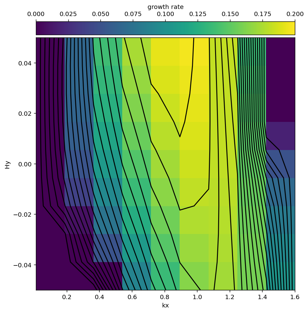
Next, we will look at the stability portrait for these parameters as a function of \(k_x\) and \(H_y\). Eigentools provides CriticalFinder as an interface for doing this. We are only going to use the grid generation function, which runs a number of eigenvalue problems at different parameters.

First, we define a set of points in each dimension, \(k_x\) and \(H_y\) using np.linspace. We then use cf.grid_generator to run an eigenvalue problem at each specified \(k_x, H_y\) point and return its growth rate. This can be run in parallel via MPI; here we’ll do a very coarse grid of just 10 by 10. This takes approximately 1 minute on a single core of a 2020 Core i7.

Because the this is a time consuming process, but plotting the data is fast and may require iteration, cf.save_grid saves the data to an HDF5 file. There is a corresponding cf.load_grid method that will load in such a file.

cf = CriticalFinder(EP, ("kx","Hy"), find_freq=False)
nx = 10
ny = 10
xpoints = np.linspace(0.01, 1.6, nx)
ypoints = np.linspace(-0.05,0.05,ny)

cf.grid_generator((xpoints,ypoints))
cf.save_grid('mixed_layer_grid')

2021-02-01 17:21:23,036 criticalfinder 0/1 INFO :: Solving Local EVP 1/100
2021-02-01 17:21:23,703 criticalfinder 0/1 INFO :: Solving Local EVP 2/100
2021-02-01 17:21:24,562 criticalfinder 0/1 INFO :: Solving Local EVP 3/100
2021-02-01 17:21:25,388 criticalfinder 0/1 INFO :: Solving Local EVP 4/100
2021-02-01 17:21:26,028 criticalfinder 0/1 INFO :: Solving Local EVP 5/100
2021-02-01 17:21:26,736 criticalfinder 0/1 INFO :: Solving Local EVP 6/100
2021-02-01 17:21:27,635 criticalfinder 0/1 INFO :: Solving Local EVP 7/100
2021-02-01 17:21:28,903 criticalfinder 0/1 INFO :: Solving Local EVP 8/100
2021-02-01 17:21:29,904 criticalfinder 0/1 INFO :: Solving Local EVP 9/100
2021-02-01 17:21:30,679 criticalfinder 0/1 INFO :: Solving Local EVP 10/100
2021-02-01 17:21:31,638 criticalfinder 0/1 INFO :: Solving Local EVP 11/100
2021-02-01 17:21:32,656 criticalfinder 0/1 INFO :: Solving Local EVP 12/100
2021-02-01 17:21:33,673 criticalfinder 0/1 INFO :: Solving Local EVP 13/100
2021-02-01 17:21:34,497 criticalfinder 0/1 INFO :: Solving Local EVP 14/100
2021-02-01 17:21:35,299 criticalfinder 0/1 INFO :: Solving Local EVP 15/100
2021-02-01 17:21:35,973 criticalfinder 0/1 INFO :: Solving Local EVP 16/100
2021-02-01 17:21:36,640 criticalfinder 0/1 INFO :: Solving Local EVP 17/100
2021-02-01 17:21:37,451 criticalfinder 0/1 INFO :: Solving Local EVP 18/100
2021-02-01 17:21:38,191 criticalfinder 0/1 INFO :: Solving Local EVP 19/100
2021-02-01 17:21:38,959 criticalfinder 0/1 INFO :: Solving Local EVP 20/100
2021-02-01 17:21:39,724 criticalfinder 0/1 INFO :: Solving Local EVP 21/100
2021-02-01 17:21:40,869 criticalfinder 0/1 INFO :: Solving Local EVP 22/100
2021-02-01 17:21:42,007 criticalfinder 0/1 INFO :: Solving Local EVP 23/100
2021-02-01 17:21:42,740 criticalfinder 0/1 INFO :: Solving Local EVP 24/100
2021-02-01 17:21:43,585 criticalfinder 0/1 INFO :: Solving Local EVP 25/100
2021-02-01 17:21:44,313 criticalfinder 0/1 INFO :: Solving Local EVP 26/100
2021-02-01 17:21:44,956 criticalfinder 0/1 INFO :: Solving Local EVP 27/100
2021-02-01 17:21:45,817 criticalfinder 0/1 INFO :: Solving Local EVP 28/100
2021-02-01 17:21:46,656 criticalfinder 0/1 INFO :: Solving Local EVP 29/100
2021-02-01 17:21:48,253 criticalfinder 0/1 INFO :: Solving Local EVP 30/100
2021-02-01 17:21:49,108 criticalfinder 0/1 INFO :: Solving Local EVP 31/100
2021-02-01 17:21:50,212 criticalfinder 0/1 INFO :: Solving Local EVP 32/100
2021-02-01 17:21:51,367 criticalfinder 0/1 INFO :: Solving Local EVP 33/100
2021-02-01 17:21:52,552 criticalfinder 0/1 INFO :: Solving Local EVP 34/100
2021-02-01 17:21:53,652 criticalfinder 0/1 INFO :: Solving Local EVP 35/100
2021-02-01 17:21:54,715 criticalfinder 0/1 INFO :: Solving Local EVP 36/100
2021-02-01 17:21:55,696 criticalfinder 0/1 INFO :: Solving Local EVP 37/100
2021-02-01 17:21:56,581 criticalfinder 0/1 INFO :: Solving Local EVP 38/100
2021-02-01 17:21:57,319 criticalfinder 0/1 INFO :: Solving Local EVP 39/100
2021-02-01 17:21:58,032 criticalfinder 0/1 INFO :: Solving Local EVP 40/100
2021-02-01 17:21:58,678 criticalfinder 0/1 INFO :: Solving Local EVP 41/100
2021-02-01 17:21:59,432 criticalfinder 0/1 INFO :: Solving Local EVP 42/100
2021-02-01 17:22:00,120 criticalfinder 0/1 INFO :: Solving Local EVP 43/100
2021-02-01 17:22:00,928 criticalfinder 0/1 INFO :: Solving Local EVP 44/100
2021-02-01 17:22:01,584 criticalfinder 0/1 INFO :: Solving Local EVP 45/100
2021-02-01 17:22:02,268 criticalfinder 0/1 INFO :: Solving Local EVP 46/100
2021-02-01 17:22:03,015 criticalfinder 0/1 INFO :: Solving Local EVP 47/100
2021-02-01 17:22:03,816 criticalfinder 0/1 INFO :: Solving Local EVP 48/100
2021-02-01 17:22:04,511 criticalfinder 0/1 INFO :: Solving Local EVP 49/100
2021-02-01 17:22:05,241 criticalfinder 0/1 INFO :: Solving Local EVP 50/100
2021-02-01 17:22:06,061 criticalfinder 0/1 INFO :: Solving Local EVP 51/100
2021-02-01 17:22:06,903 criticalfinder 0/1 INFO :: Solving Local EVP 52/100
2021-02-01 17:22:07,797 criticalfinder 0/1 INFO :: Solving Local EVP 53/100
2021-02-01 17:22:08,579 criticalfinder 0/1 INFO :: Solving Local EVP 54/100
2021-02-01 17:22:09,647 criticalfinder 0/1 INFO :: Solving Local EVP 55/100
2021-02-01 17:22:11,107 criticalfinder 0/1 INFO :: Solving Local EVP 56/100
2021-02-01 17:22:12,370 criticalfinder 0/1 INFO :: Solving Local EVP 57/100
2021-02-01 17:22:14,074 criticalfinder 0/1 INFO :: Solving Local EVP 58/100
2021-02-01 17:22:15,182 criticalfinder 0/1 INFO :: Solving Local EVP 59/100
2021-02-01 17:22:16,132 criticalfinder 0/1 INFO :: Solving Local EVP 60/100
2021-02-01 17:22:16,914 criticalfinder 0/1 INFO :: Solving Local EVP 61/100
2021-02-01 17:22:17,628 criticalfinder 0/1 INFO :: Solving Local EVP 62/100
2021-02-01 17:22:18,385 criticalfinder 0/1 INFO :: Solving Local EVP 63/100
2021-02-01 17:22:19,116 criticalfinder 0/1 INFO :: Solving Local EVP 64/100
2021-02-01 17:22:19,870 criticalfinder 0/1 INFO :: Solving Local EVP 65/100
2021-02-01 17:22:20,858 criticalfinder 0/1 INFO :: Solving Local EVP 66/100
2021-02-01 17:22:21,823 criticalfinder 0/1 INFO :: Solving Local EVP 67/100
2021-02-01 17:22:22,602 criticalfinder 0/1 INFO :: Solving Local EVP 68/100
2021-02-01 17:22:23,660 criticalfinder 0/1 INFO :: Solving Local EVP 69/100
2021-02-01 17:22:24,525 criticalfinder 0/1 INFO :: Solving Local EVP 70/100
2021-02-01 17:22:25,514 criticalfinder 0/1 INFO :: Solving Local EVP 71/100
2021-02-01 17:22:26,515 criticalfinder 0/1 INFO :: Solving Local EVP 72/100
2021-02-01 17:22:27,298 criticalfinder 0/1 INFO :: Solving Local EVP 73/100
2021-02-01 17:22:28,001 criticalfinder 0/1 INFO :: Solving Local EVP 74/100
2021-02-01 17:22:28,686 criticalfinder 0/1 INFO :: Solving Local EVP 75/100
2021-02-01 17:22:29,308 criticalfinder 0/1 INFO :: Solving Local EVP 76/100
2021-02-01 17:22:29,997 criticalfinder 0/1 INFO :: Solving Local EVP 77/100
2021-02-01 17:22:30,666 criticalfinder 0/1 INFO :: Solving Local EVP 78/100
2021-02-01 17:22:31,340 criticalfinder 0/1 INFO :: Solving Local EVP 79/100
2021-02-01 17:22:32,074 criticalfinder 0/1 INFO :: Solving Local EVP 80/100
2021-02-01 17:22:32,827 criticalfinder 0/1 INFO :: Solving Local EVP 81/100
2021-02-01 17:22:33,418 criticalfinder 0/1 INFO :: Solving Local EVP 82/100
2021-02-01 17:22:34,105 criticalfinder 0/1 INFO :: Solving Local EVP 83/100
2021-02-01 17:22:34,854 criticalfinder 0/1 INFO :: Solving Local EVP 84/100
2021-02-01 17:22:35,509 criticalfinder 0/1 INFO :: Solving Local EVP 85/100
2021-02-01 17:22:36,269 criticalfinder 0/1 INFO :: Solving Local EVP 86/100
2021-02-01 17:22:37,080 criticalfinder 0/1 INFO :: Solving Local EVP 87/100
2021-02-01 17:22:37,947 criticalfinder 0/1 INFO :: Solving Local EVP 88/100
2021-02-01 17:22:38,731 criticalfinder 0/1 INFO :: Solving Local EVP 89/100
2021-02-01 17:22:39,591 criticalfinder 0/1 INFO :: Solving Local EVP 90/100
2021-02-01 17:22:40,567 criticalfinder 0/1 INFO :: Solving Local EVP 91/100
2021-02-01 17:22:41,374 criticalfinder 0/1 INFO :: Solving Local EVP 92/100
2021-02-01 17:22:41,926 criticalfinder 0/1 INFO :: Solving Local EVP 93/100
2021-02-01 17:22:42,579 criticalfinder 0/1 INFO :: Solving Local EVP 94/100
2021-02-01 17:22:43,411 criticalfinder 0/1 INFO :: Solving Local EVP 95/100
2021-02-01 17:22:44,064 criticalfinder 0/1 INFO :: Solving Local EVP 96/100
2021-02-01 17:22:44,751 criticalfinder 0/1 INFO :: Solving Local EVP 97/100
2021-02-01 17:22:45,445 criticalfinder 0/1 INFO :: Solving Local EVP 98/100
2021-02-01 17:22:46,123 criticalfinder 0/1 INFO :: Solving Local EVP 99/100
2021-02-01 17:22:47,000 criticalfinder 0/1 INFO :: Solving Local EVP 100/100

Finally, we produce a plot comparable to the left panel of figure 6 in Boccaletti, Ferrari, & Fox-Kemper (2007).

pax,cax = cf.plot_crit()
pax.collections[0].set_clim(0,0.2)
cax.xaxis.set_ticks_position('top')
cax.xaxis.set_label_position('top')
contours = np.linspace(0,0.2,20,endpoint=False)
pax.contour(cf.parameter_grids[0], cf.parameter_grids[1],cf.evalue_grid.real, levels=contours, colors='k')
pax.figure.savefig('mixed_layer_growth_rates.png',dpi=300)