Getting Started

eigentools comes with several examples to get you started, but let’s outline some basics in a very simple problem, the 1-D wave equation with \(u = 0\) at both ends. This is not quite as trivial a problem as it might seem, because we are expanding the solution in Chebyshev polynomials, but the eigenmodes are sines and cosines.

from eigentools import Eigenproblem
import dedalus.public as de

Nx = 128
x = de.Chebyshev('x',Nx, interval=(-1, 1))
d = de.Domain([x])

string = de.EVP(d, ['u','u_x'], eigenvalue='omega')
string.add_equation("omega*u + dx(u_x) = 0")
string.add_equation("u_x - dx(u) = 0")
string.add_bc("left(u) = 0")
string.add_bc("right(u) = 0")

EP = Eigenproblem(string)
EP.solve(sparse=False)
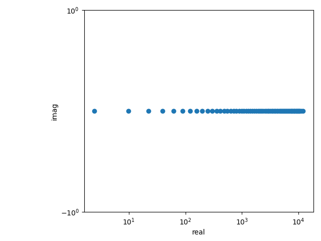
ax = EP.plot_spectrum()
print("there are {} good eigenvalues.".format(len(EP.evalues)))
ax.set_ylim(-1,1)
ax.figure.savefig('waves_spectrum.png')

ax = EP.plot_drift_ratios()
ax.figure.savefig('waves_drift_ratios.png')

That code takes about 10 seconds to run on a 2020 Core-i7 laptop, produces about 68 “good” eigenvalues, and produces the following output:

eigentools has taken a Dedalus eigenvalue problem, automatically run it at 1.5 times the specified resolution, rejected any eigenvalues that do not agree to a default precision of one part in \(10^{-6}\) and plotted a spectrum in six extra lines of code!

Most of the plotting functions in eigentools return a matplotlib axes object, making it easy to modify the plot defaults. Here, we set the y-limits manually, because the eigenvalues of a string are real. Try removing the ax.set_ylim(-1,1) line and see what happens.

Mode Rejection

One of the most important tasks eigentools performs is spurious mode rejection. It does so by computing the “drift ratio” [Boyd2000] between the eigenvalues at the given resolution and a higher resolution problem that eigentools automatically assembles. By default, the “high” resolution case is 1.5 times the given resolution, though this is user configurable via the factor keyword option to Eigenproblem().

The drift ratio \(\delta\) is calculated using either the ordinal (e.g. first mode of low resolution to first mode of high resolution) or nearest (mode with smallest difference between a given high mode and all low modes). In order to visualize this, EP.plot_drift_ratios() in the above code returns an axes object making a plot of the inverse drift ratio (\(1/\delta\)),

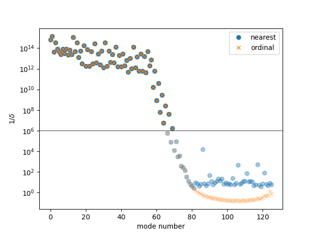
Good modes are those above the horizontal line at \(10^{6}\); bad modes are also grayed out. In this case, the nearest and ordinal methods produce identical results. If the problem contains more than one wave family, nearest typically fails. For an example, see the MRI example script. Note that nearest is the default criterion used by eigentools.

Boyd2000

Boyd, J (2000). “Chebyshev and Fourier Spectral Methods.” Dover. http://www-personal.umich.edu/~jpboyd/aaabook_9500toc.pdf